Tutorial G(t) Application

Fitting Maxwell modes to G(t) from MD simulations

1. Start RepTate and create a new Gt Application :

   

2. Drag and drop a file(s) with a .gt extension. In this case, we will use the file C0224_NVT_450K_1atm.gt e.g. the set of data/Gt/PI_**k_T-35.tts included in the distribution, which corresponds to the relaxation modulus of atomistic MD simulations of linear polyethylene with molecular weight approximately 3 kDa (corresponding to 224 carbon atoms in the backbone). See Data Files for a description of the data file organization.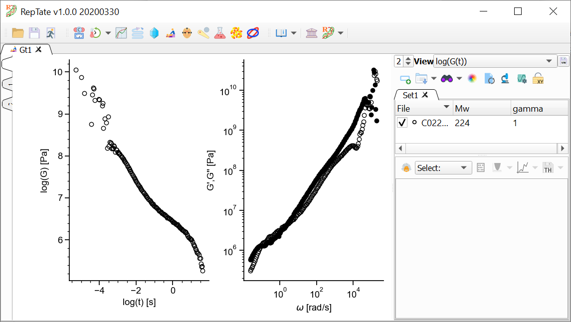

   

By default, 2 views are shown:

• The relaxation modulus log(G(t)) vs log(t)

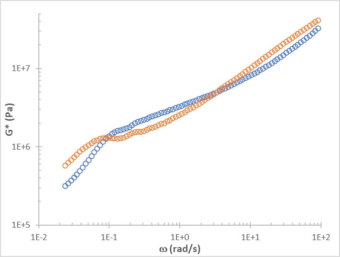
• The complex modulus G*(w), calculated using the i-Rheo algorithm.

1. Select a theory, e.g. “Maxwell modes”, and press to create it (calculation is done with default parameter values). Press “Minimize Error” .

   

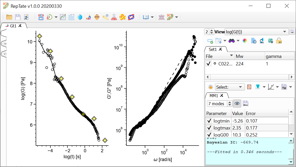
2. The MD data has too many oscillations at early time, so we want to avoid fitting data for t<1e-4. First, we are going to restrict the xrange of the data that we are going to fit.

   

3. In addition, we want the longest mode to be representative of the terminal time, and the shortest time to be inside our x-range. We can drag the first and last modes and stretch or shrink the modes like an accordion, then press Fit again:

   

4. In order to save the theory results, we have several options available.

   • To save the theory line(s), click the button. This option, saves the theory prediction exactly in the same format as the original data file, i.e. in a two-column file with t and G(t).

   • If we want to save the spectrum of Maxwell modes, click the button. This will save a text file with data similar to the example shown below. From the spectrum Maxwell modes it is very easy to build both the predicted G(t) and the complex modulus G*(w):

     # Maxwell modes
     # Generated with RepTate v1.0.0 20200330
     # At 12:58:24 on Mon May 11, 2020
     
     #number of modes
     7
     
     #   i            tau_i             G_i
        1         0.0013869     1.42029e+08
        2        0.00691551     4.45053e+07
        3         0.0344828     1.06538e+07
        4          0.171941     3.45984e+06
        5          0.857349     1.58526e+06
        6             4.275     1.15323e+06
        7           21.3164     1.39205e+06
     
     #end
     

   • If we want to save the complex modulus G*(w), we can click the button. This option will create a text file with all the experimental data as shown in the current view or set of views. In the example shown above, we would get a file with contents similar to what is shown below. The file has 5 columns (the first two correspond to the first view and the last three columns correspond to the second view, the complex modulus calculated with i-Rheo):

     #view(s)=[log(G(t)), i-Rheo G',G'', i-Rheo-Over G',G'', Schwarzl G',G''];ncontri=1.0;Mw=224.0;gamma=1.0;
     log(t)                 log(G)          $\omega$        G'              G''
     -inf                   1.01077051e+01  2.38418806e-02  3.12414178e+05  5.86601932e+05
     -5.30103000e+00        1.00546207e+01  2.62151862e-02  3.37632680e+05  6.38890093e+05
     -5.00000000e+00        9.87919397e+00  2.88247391e-02  3.67555611e+05  6.94478070e+05
     -4.82390874e+00        9.48972792e+00  3.16940561e-02  4.02919022e+05  7.53142734e+05
     

   • In order to obtain the i-Rheo complex modulus for the theory prediction, the procedure is a little longer, but still very easy. Right-click on the G’ curve corresponding to the theory (continuous line) and copy the data to the clipboard. Then, you can paste it in Microsoft Excel or whichever software you want. Repeat the procedure with the G’’ curve (dashed line in the example) and paste the data in Excel. You should end up with data as shown below (the omega column is repeated, so you can get rid of it).

     

   • The data can also be pasted into a text file which, with the right tts extension, can be imported into the LVE app of RepTate.