General Description of RepTate

RepTate (Rheology of Entangled Polymers: Toolkit for Analysis of Theory & Experiment) is a software package for viewing, exchanging and analysing experimental data. Several of the classical and latest theories of polymer dynamics are included in RepTate, so they can be tested and fitted to the experimental data.

The software is designed in a modular way, so it is easy to extend to analyze new types of data and fit with new theories.

RepTate makes extensive use of the following packages and libraries:

• Matplotlib: Text [1].

• Scipy: Text [2].

• Numpy: Text [3].

• Qt and Pyqt: Text [4], Text [5].

Main RepTate Window

The main RepTate window is called the Application Manager and is a multiple document interface (MDI) (see Fig. 1). All the applications can be opened from the Application Manager and will reside inside it. At the top of the Application Manager there is a toolbar that allows to open different applications (label 1 in Fig. 1), load and save RepTate projects, read the help and exit RepTate. Currently open applications can are shown as tabs below the toolbar (label 2 in Fig. 1). By default, tabs are named after the application name and a number. The name can be changed by double-clicking on the tab.

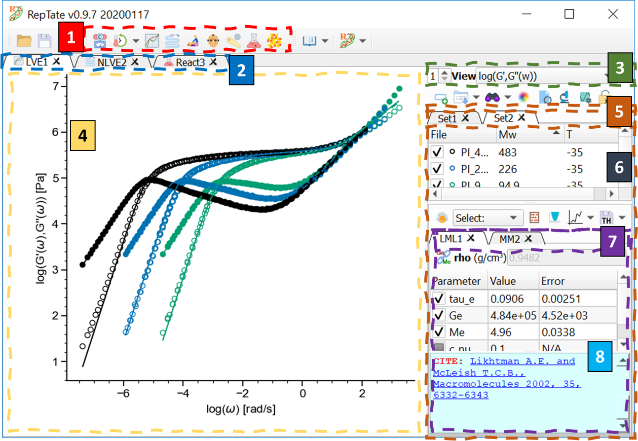
Fig. 1 Main RepTate window showing the most important elements in the user interface.

Applications have three main separate areas:

• The plot, in the center, is where the experimental data files and theoretical fits are shown (label 4 in Fig. 1).

• A vertical region at the right of the window, that allows to:

  • Select the current View (way of representing the data, label 3 in Fig. 1)

  • Open data Files and arrange them into different Datasets (label 5 in Fig. 1). Different Datasets are shown as tabs, named by default as “Set” + number. The name of a Dataset can be changed by double-clicking on the tab.

  • Create a Theory associated to a given Dataset and fit it (minimize the error with respect to the Files within that Dataset, label 7 in Fig. 1). Currently open theories are named after the theory name + a number. The name can be changed by double-clicking on the tab.

Files in the current DataSet are shown in a table, along with the main parameters that describe each file (label 6 in Fig. 1). Files can be added to a Dataset with the “Open Data File” button (Ctrl+O) or by dragging them from the file explorer and dropping them on the RepTate window. In the Theory area, the parameters of the current theory are shown in a table, with their current value and error. A blue box below the table shows information during the calculation and fitting procedure (label 8 in Fig. 1)

By clicling on the “Data Inspection” button (label 1 in Fig. 2), a new region on the left of the plot area is shown where the user can inspect the contents of a file, shift data and use the Tools. Two separate areas are shown:

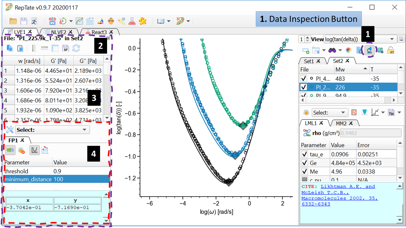
Fig. 2 Extended RepTate window showing file data and Tools.

• A region (label 3 in Fig. 2) where the file contents are shown in a table. Above the table (label 2 in Fig. 2) there is a toolbar that allows the user to do some operations on the data (copy, paste, shift, etc).

• A region (label 4 in Fig. 2) that lets the user apply different Tools to the current Dataset.

The data inspection and Tools region is hidden by default.

Operating with Datasets

When an new application is opened, a new tab is created in the Main RepTate window, showing an empty application with an empty dataset, no theories and the default view. New data files must be added to the dataset in order to use all the functionality of RepTate.

Structure of data files

Only text files that have the right extension and contain the expected data can be added to the current application. The general structure of the text files that can be read by RepTate is as follows (see the example below for a quick reference):

• [Required] The first line contains a list of parameters that describe the contents of the data in the file, as a list of variables and values separated by semicolons. Typically, the parameters will describe the conditions (temperature, pressure, etc) at which the experiment was done, plus some additional parameters to characterize the material (chemistry, molecular weight, etc) and the author of the data. Some parameters are needed by some applications and theories (for example, the temperature in the TTS module) and RepTate will show a warning if their values are missing. The values of the parameters can be real numbers, integers or strings.

• [Optional] Some additional text lines may be present in the file with further info about the experimental data (the date and location where the data was taken, the equipment, etc). These lines ignored by RepTate.

• [Required] The data itself must be stored in the file as columns separated by spaces or tabs. The number of columns must be greater or equal than the number of columns required by the application, and in the expected order. Additional columns are discarded. For more information, check the documentation for each particular application.

var1=value1;var2=value2;var3=value3;...
Some text
# Some text
1.90165E+0      7.38023E+1      1.35152E+4
3.01392E+0      1.99063E+1      2.14834E+4
4.51700E+0      3.72861E+1      3.17756E+4
...             ...             ...

For more info about valid extensions and data structure inside the files, check the documentation for each application.

Adding files to datasets

There are two ways to add Files to the current application:

• By dragging and dropping them from the system file explorer to the Application window (see Fig. 3).

• By pressing the Open Data File button (Ctrl+O). A file dialog is shown where one file or more files of the right type can be selected.

Fig. 3 Dragging and dropping some files to the RepTate window.

Importing data from Excel files

This feature is experimental and will be improved in the future. In the current version, when the user selects the button “Import from Excel” , under the button menu, a dialog is shown that allows the user to (see Fig. 4):

• select the Excel file

• set the file parameters

• select Excel Sheet that contains the data

• set the number of rows in the Excel sheet that must be skipped

• set the columns in the Excel sheet that correspond to the columns that the RepTate application expects to read.

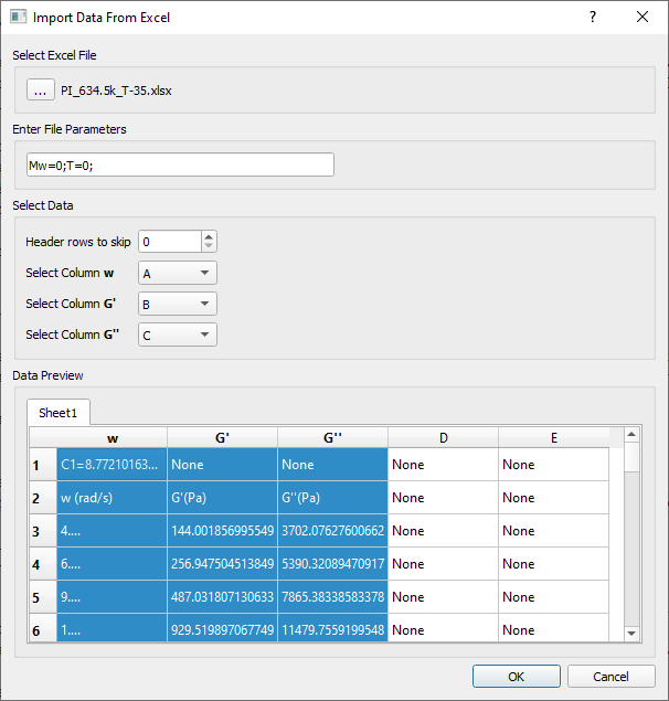
Fig. 4 Importing data from an Excel file into the LVE application.

Sorting Files in a Dataset

The files in a Dataset can be sorted by name or parameter value, in increasing and decreasing order, by clicking in the corresponding column header. Clicking several times on the same header will invert the sorting order. A small arrow next to a column header name will indicate how the files in the current Dataset are sorted (see Fig. 5).

If a Dataset column corresponds to a unit-aware file parameter, right-clicking that column header opens a pop-up menu with the registered compatible units for that quantity. Selecting one changes the display unit for that parameter in the current Dataset only.

If the current plot view has unit-aware axes, right-clicking on the plot area also opens axis-unit menus for the current x and y axes whenever compatible alternative units are available. Selecting one changes the display unit for the current view axis, updates the axis label, and replots all visible data and theory curves in that view.

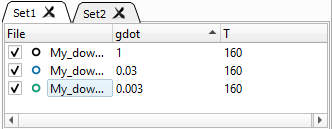
Fig. 5 A Dataset with files sorted by decreasing value of the gdot parameter.

When the files in a Dataset are sorted, the colours assigned to each file are also changed. The order of the colours is assigned by the selected palette. The number of colours in some palettes is limited and, therefore, if the number of files exceed the number of colours available, some files may end up having the same colour.

Viewing/Hiding Files

Each file in a Dataset can be in the enabled (checked) or disabled state (unchecked, see Fig. 6). When files are disabled, they are not shown in the current view and they are not considered during theory calculation and fitting.

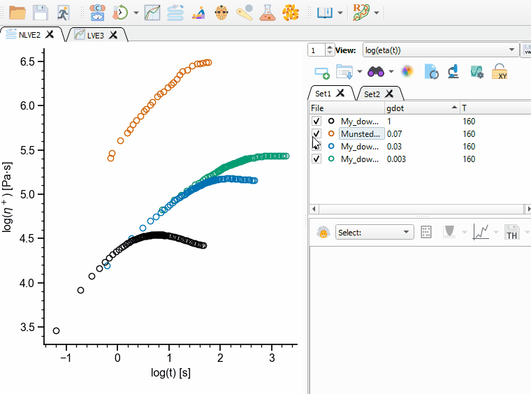
Fig. 6 Enabling/disabling files in a Dataset.

Showing/Editing file parameters

By double-clicking on a file name in the Dataset area, it is possible to view/edit the parameters of the file. A dialog will open, where all the file parameters are shown and all their values can be viewed/edited.

Creating new datasets

Sometimes, it is convenient to load data into separate data sets, because the data correspond to different materials or the experiments have been done in different conditions. In order to create a new empty dataset, the user must click on the “Create an empty DataSet” button (Ctrl+N) in the DataSet toolbar. By default, new DataSets are named Set i, where i is an integer that starts from 1 and increments as new DataSets are opened. The DataSet name can be changed by double-clicking on the DataSet tab.

When there are more than one Dataset in the current application, the user can switch Datasets by clicking on the corresponding tab. By default, RepTate only plots the data in the currently active Dataset. If the button “View all Datasets simultaneously” button is clicked, all the data in all open Datasets is shown.

Adding Dummy files to datasets

In some cases, the user may want to explore the results of a given theory but he/she does not have any experimental data files available. Since the theories are only applied to the active files of the Dataset that owns the theory, it is convenient to be able to create empty files with parameters that span some range of values of interest (for example, the user may be interested in exploring the results of some theory when the molecular weight of the samples is changed). In RepTate, this can be done by adding Dummy files, in the submenu under the “Open Data File” button.

When the “Add Dummy files” button is clicked, a dialog is shown allowing the user to configure how the files are going to be generated (see Fig. 7):

• The parameter(s) that are going to be changed systematically in the dummy files. By default, the possible parameters are selected from the list of important parameters, defined for every application. By ticking the check-box next to a parameter, it is selected.

• The range of values over which the parameter will be swept, which is defined by a minimum value, a maximum value, the number of points and scale (linear or logarithmic) that will be used to separate the points between the minumum and the maximum.

• The data in the dummy files is arbitrary. The user can select the range, number of points and scale (linear or log) in the dummy file for the first column (which frequently will act as the x-coordinate in views), as well as the default y value for the remaining columns.

• The user can also input the chemistry, which may be interesting if a certain material is available in the Materials Database.

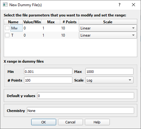
Fig. 7 Dialog for adding Dummy files to a DataSet.

Reloading the data

Some times, the user may be representing some data that is being updated in real time (because an experiment or simulation is running at the same time as the RepTate session). In this cases, it is interesting to update the data in RepTate by reading again the file. This can be done by clicking the button “Reload Data Files & Theories” (Ctrl+R).

When reloading data files, RepTate also refreshes unit-aware file parameters from the file header, including changes in both value and unit, and updates the Dataset display accordingly.

Operating with Views

The data read from the files can be represented in several different ways, which are different for each application. In RepTate, the way some experimental or theory data are represented is referred to as the View.

There are two different ways to select a View:

• From the drop-down box at the top-right corner of the Application window. By clicking on the box, a menu is shown with all the Views that are defined in the current application. By hovering the mouse over the View names, some additional information may be displayed.

• By right-clicking on the plot area, a menu is displayed.

At the left of the drop-down box, there is a small up-down selector that allows the user to change the number of graphs that are shown in the plot area. When there are more than one graph, a small set of tabs is shown on the left of the Plot area (see Fig. 8). The number of tabs is equal to the number of Views + 1. The tab 0 shows all views and the other tabs show a single view.

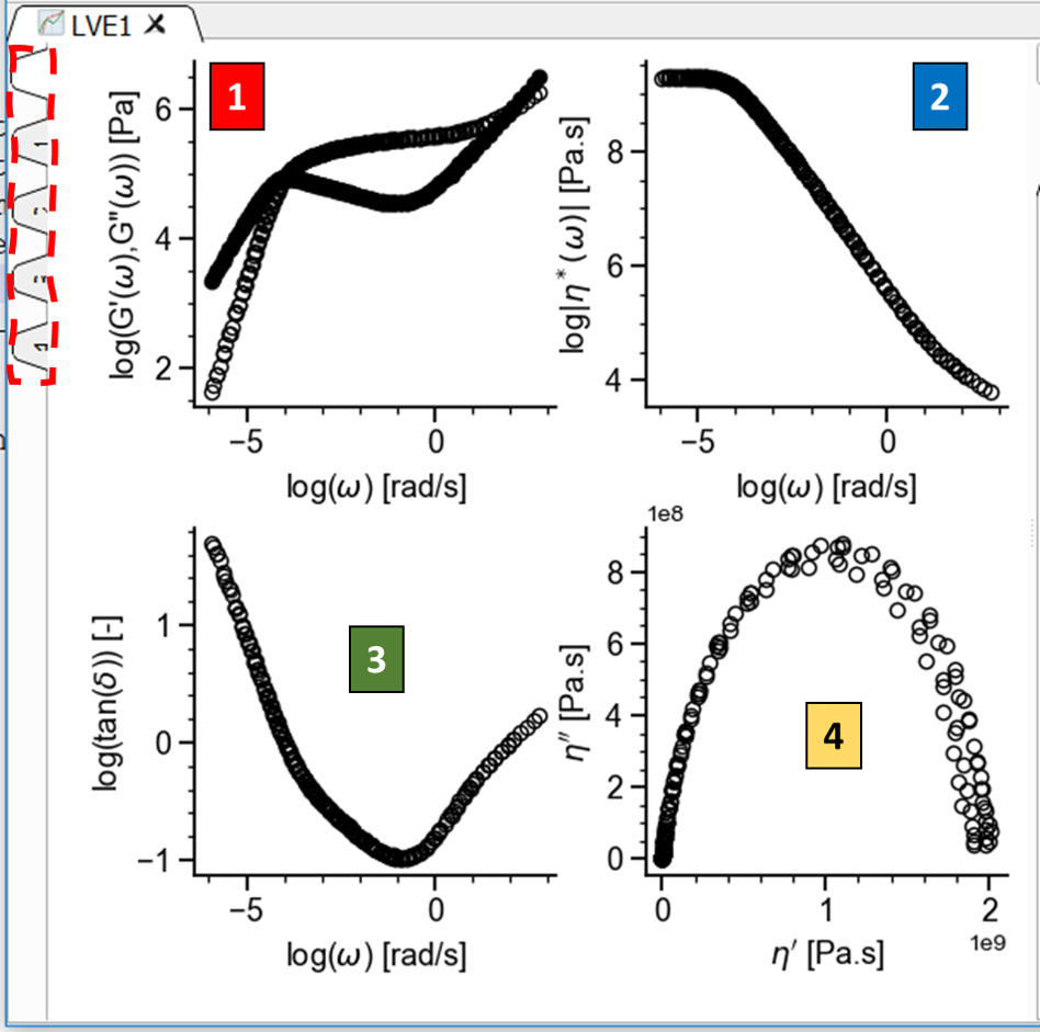
Fig. 8 Plot area showing 4 different views and the tabs to switch from all to particular views (left).

Most Applications in RepTate show just one graph by default.

The data, as represented by the current View/Views, can be saved to a text file by clicking on the button at the right of the View combo box.

Plot Area

The plot area shows the graphical representation of the data files in the current Dataset (or all the Datasets in the current application, if the “View all Datasets simultaneously” button is clicked). Several operations can be done in the plot area:

• By clicking on a data point, a label is shown with its (\(x\), \(y\)) coordinates, with respect to the current View (label 1 in Fig. 9). The label can be hidden by clicking on it again.

• By right-clicking on the plot area and dragging the mouse, the user can zoom to an specific region of the plot.

• By using the mouse wheel, the user can zoom in or out in the plot.

• By right-clicking on the plot, a menu is shown with the following operations (label 3 in Fig. 9):

  • The chart can be copied to the clipboard as an image. The image can be pasted on any other program (such as Microsoft Word or Powerpoint)

  • The chart can be saved to an image file, using different formats (png, pdf, etc).

  • An annotation label can be added to the plot (label 2 in Fig. 9). LaTeX commands can be used in the text of the annotation. Annotation labels can be moved around by dragging them with the mouse and edited by double-clicking on them.

  • The view can be reset to the default zoom.

  • The view can be changed to any of the available views in the current application.

  • If the current view uses unit-aware axes, the display unit of the x and y axes can be changed from the corresponding axis-unit submenus. RepTate then updates the axis label and replots the visible data and theory in the selected units.

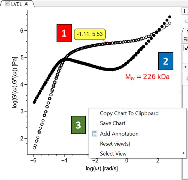
Fig. 9 Plot area showing data point coordinates (1), annotations (2) and pop-up menu (3).

Additional view options can be set by clicking on the “Show/Hide Figure Toolbar” button on the Dataset area. The x-y ranges can be fixed by clicking on the “Lock XY axes” in the Dataset area.

Changing the Plot Properties

Most of the visual aspects of the plot (lines, symbols, axes labels, legend, etc) can be changed, by clicking the “Plot Settings” button (Ctrl+M) in the Dataset area. A dialog is shown with different tabs, each one dedicated to a different aspect of the plot.

• Data: in this tab, the user can select how the experimental data loaded in the Dataset is shown on the current view (see Fig. 10). By default, the experimental data is always shown as symbols, and the user can select the symbol type, size and colour. The different files in the Dataset can be shown with the same or different symbols and the colour can be set by selecting from a list of available colour palettes. Alternatively, the color can be fixed for all files or selected from a gradient, interpolating from Colour1 (which is used for the first file in the current Dataset) to Colour2 (for the last file).

Fig. 10 Changing the Plot properties of the data.

• Theory: the line type, width and colour can be selected (fixed or the same colour as the data).

• Legend: here, the user can select if he/she wants to show the legend in the current plot, along with its location, font and other properties

such as the label that will be used to represent the data (see Fig. 11). For example, if the files in the current Dataset have the parameter Mw defined with a value, it can be used as the legend label by filling the Legend Labels field with the text “Mw = [Mw]”.

• Annotations: here, the default properties of annotations (colour, font, opacity, etc) can be set. All new notations will have these properties. Individual annotation properties can be changed by double-clicking on the text of a particular annotation.

Fig. 11 Changing the style of the legend.

• Axes: the font of the labels and the colour of the labels and axes can be changed. Also, the user can choose whether to show grid lines or not.

As an example, a plot of LVE data with different graphical settings is shown in Fig. 11.

Fig. 12 Example of a plot of LVE data where some of the default graphical properties have been changed.

Inspecting the Data

When the user clicks the button “Inspect contents of data files” (Ctrl+I) in the Dataset area, a new panel is shown on the left side of the application window. In this panel, some operations can be done on the data, like checking the contents, copy and pasting data, shifting the curves around by dragging them with the mouse or applying Tools to the data.

View the current file data

When a file in the current Dataset is selected with the mouse, the corresponding plot is highlighted and the contents of the file are shown in the data inspection table (if the data inspection table is shown, see Fig. 13).

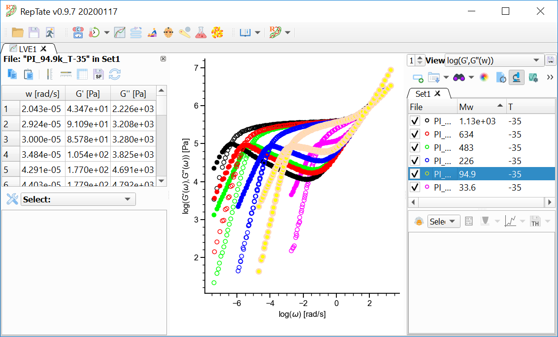
Fig. 13 Inspecting the contents of the selected file.

Copy/Paste data

The data shown in the inspection data table can be copied as text (columns separated by tabs) by selecting the corresponding cells, columns or rows from the table and pressing the button “Copy” in the data inspaction area. The copied data can be pasted in another application like Excel or Matlab, or even to a different file by pressing the button “Paste” in the data inspection area.

Shift the data

Sometimes it may be convenient to compare features of two different data files that are represented in the same plot. For example, one may be interested in comparing the different terminal regions of G’ data of samples of the same polymer with different molecular weight. RepTate allows the user to shift the data vertically and/or horizontally by pressing the buttons “Shift the selected curve vertically” and/or “Shift the selected curve horizontally” 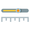, respectively, in the data inspection area. Once the user finishes shifting the curves, he/she can check, save and reset the values of the shift factors by clicking on the corresponding buttons in the data inspection area. The whole procedure is summarized in Fig. 14.

Fig. 14 Shifting some curves horizontally and viewing the shift factors.

When the axis with respect to which the shifting is being carried out is in logarithmic scale, the shift factor represents the decimal logarithm of the factor by which one should multiply the data in order to obtain the observed shift. When the axis is in linear scale, the shift factor is just the linear shift needed to obtain the observed shift.

Fitting a theory

One of the most important features of RepTate is the ability to easily fit a theory to a set of experimental data files. The available theories in each RepTate application are described and discussed in the documentation corresponding to each application. Here, we give a short summary of the general ideas about how theories are handled in RepTate.

It is important to note that, in RepTate, theories belong to Datasets, i.e. they are applied only to the data files in the Dataset under which the theory was created.

Opening a new Theory

Below the Dataset table that contains the files, there is a toolbar for operating with theories. First, the user should select a theory from the list available in the drop-down menu. Once the right theory is selected, a new instance of the theory can be created by clicking on the “Create Selected Theory” button (Alt+N). New theories are shown as tabs below the theory toolbar. By default, theories are named after a combination of capital letters selected after the theory name + an index number. The name of any theory can be changed by double clicking on the corresponding tab.

Viewing/Editing Parameter values and options

When a new theory instance is created, a new tab opens in which two clearly separate areas can be seen (see Fig. 15):

• A table that lists the parameters of the theory, with their current value and, if the theory has been fitted to some experimental data, the error of the fitting.

• A text area with a light blue background that shows all the relevant information during the calculation and fitting of the theory, as well as any citation information that is relevant to the current theory.

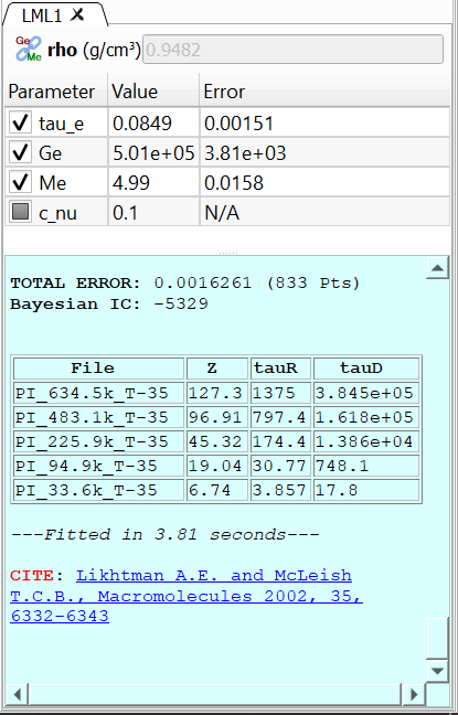
Fig. 15 A theory with the parameters table and the log area (with cyan background).

Theory parameters can be shown in the table in three possible states:

• Checked: the parameter value will be optimized during the fitting procedure.

  • Unchecked: the value of the parameter will not be optimized (it will remain constant during the next fitting procedure).

  • Grayed out or partially checked: the parameter cannot be optimized. This is intended for parameters, like exponents of scaling factors, that take well known values. Typically, grayed parameters take their value from a set of prescribed discrete values.

Theory parameters have properties, and some of these properties are very important during theory fitting. In order to check and edit the properties of parameters, the user can double-click on any parameter name. Then, a dialog is shown with a tablist, with a tab for each parameter of the theory and the current properties of each parameter (see Fig. 16). The most important properties of a parameter are:

• name: the short name of the parameter. It is hardcoded into the theory and cannot be changed.

• description: a short description of the parameter. It is hardcoded into the theory and cannot be changed.

• type: the numerical type of the value of the parameter. It can be real, integer, discrete_real (its value is selected from a discrete list of real values), discrete_integer (discrete list of integer values) and boolean.

• opt_type: indicates whether the parameter value will be optimized during the fitting procedure or not. Possible states are: opt (will be optimized), nopt (will not be optimized) and const (cannot be optimized).

• min_value: minimum value that the parameter can adopt. If the parameter is not bounded, the minimum value is -inf.

• max_value: maximum value that the parameter can adopt. If the parameter is not bounded, the maximum value is inf. The bounds should not be exceeded during minimization. If the user inputs manually a value that is outside the bounds, RepTate will issue a warning and set the parameter value to the bound that has been exceeded.

• display_flag: whether the parameter will be shown in the parameter table or not.

• discrete_values: comma-separated list of values that the parameter can adopt. Only relevant if the parameter type is either discrete_real or discrete_integer.

• quantity, internal_unit and display_unit: unit metadata for unit-aware parameters. The parameter value used by the theory is stored in internal_unit. The value shown in the table is converted to display_unit. If compatible units are registered, display_unit can be changed from the parameter-properties dialog without changing the stored physical value.

For unit-aware parameters, editing the value in the theory table uses the display unit shown next to the parameter name. For example, a parameter stored internally in kg/mol may be displayed and edited in Da; RepTate converts the entered value back to kg/mol before the calculation.

Fig. 16 Dialog for viewing/editing parameter properties.

Calculating the theory

When the button “Calculate Theory” (Alt+C) is pressed, the theory is calculated using the current values of the theory parameters and for all the files in the current dataset. Since the theory may use some of the file parameters, the result of applyting the theory to each files will be different. By default, the theory is calculated exactly in the same x points as the corresponding data file. This can be changed by editing the file parameters and selecting “Extra Theory Range”.

When the theory calculation is done, some interesting information is shown in the theory log area (see Fig. 17). By default, the information displayed contains:

• A table with the list of files that theory has been applied to, with the selected error measure and the number of points of each file.

• The total error (the weighted mean of the file errors) and the total number of points.

• The Bayesian Information Criterion (BIC), always evaluated from the non-normalized mean squared error as \(BIC = n \log(MSE)+ p\log(n)\), where n is the number of data points and p is the number of free fitting parameters. In general, the model with the lowest BIC value should be preferred.

• Some additional information may be shown by some theories (for example, in Fig. 17, the Likhtman-McLeish theory shows some tube related values for each file).

• The time it took to calculate the theory, in seconds.

• The relevant literature that the user should cite if he/she intends to use the results from the theory. The journal articles are shown as links that can be clicked in order to visit the publisher web.

Error calculation options

The error calculation options are available from the Calculate Theory button menu. The checkbox Normalize by experimental data controls whether residuals are divided by the experimental data before the error is computed. The Error norm option controls whether squared residuals or absolute residuals are averaged. The four combinations are reported in the theory log using the following labels:

• MSE: \(\mathrm{mean}((y_\mathrm{th} - y_\mathrm{exp})^2)\)

• MSRE: \(\mathrm{mean}(((y_\mathrm{th} - y_\mathrm{exp}) / y_\mathrm{exp})^2)\)

• MAE: \(\mathrm{mean}(|y_\mathrm{th} - y_\mathrm{exp}|)\)

• MRAE: \(\mathrm{mean}(|(y_\mathrm{th} - y_\mathrm{exp}) / y_\mathrm{exp}|)\)

The default is the historical squared, non-normalized error (MSE).

Fig. 17 Example of the information displayed after a theory calculation is finished.

Fitting the theory

Use the Minimize Error button in the theory toolbar, or press Alt+M, to fit the currently active theory tab to the active files in the current dataset. Fitting changes only the parameters that are checked in the theory parameter table; unchecked parameters keep their current values, and grayed parameters cannot be optimized.

The fit uses the data as shown in the current view. Hidden files are ignored. For theories that can only use one file, RepTate warns if more than one file is active and then uses the highlighted file, or the first active file if no file is highlighted.

When fitting starts, RepTate writes a Parameter Fitting section in the theory log. If graphical x- or y-range limits are visible, the selected ranges are reported there and only points inside those ranges are used. Points with NaN or infinite values are excluded from the fit.

During a fit, the Minimize Error button changes to a stop button. Pressing it again requests the current fit to stop. If a theory calculation is already running, RepTate does not start a fit and reports that the theory is busy calculating.

After a successful fit, the optimized parameter values are stored in the active theory, the parameter table is updated, and the theory is recalculated with the fitted parameters. The log reports the initial and final error, the number of function evaluations, the fitted parameter values with estimated errors when available, the elapsed fitting time, and any citation information supplied by the theory.

How the fitting is done

During fitting, RepTate minimizes the selected error between the active theory prediction and the selected experimental data. The experimental data are first converted through the current application view, so fitting is performed on the same coordinates that are displayed in the plot. Only active files are used. If x- or y-range fitting limits are visible, only points inside those ranges are included. Points with NaN or infinite x or y values are ignored.

The optimizer changes only the theory parameters that are checked in the parameter table. Unchecked parameters keep their current values, and grayed parameters cannot be selected for fitting. The starting values are the current parameter values. The minimum and maximum values in the parameter properties are passed to the fitting method as bounds, and integer parameters are marked as integer-valued where the selected method supports this.

For each trial set of parameter values, RepTate recalculates the theory and compares the resulting prediction with the selected experimental points. The error measure is the one selected in the error-calculation options: squared or absolute residuals, with optional normalization by the experimental data. If normalization by experimental data is selected and the fitting data contain zero values, the fit is stopped because the relative error cannot be evaluated.

The default LS method is a local fit starting from the current parameter values. The global fitting methods first search more broadly over the allowed parameter bounds, then RepTate refines the result with a local fitting step before storing the final parameters. A fit can still depend on the chosen starting values, parameter bounds, data range, error measure, and fitting method; RepTate does not guarantee that a global optimum has been found. Individual theories may also extend or override parts of the generic calculation.

When fitting finishes successfully, the active theory parameters are updated, the theory is recalculated with the fitted values, and the plot is refreshed. The theory log reports the fitting method, any active fitting ranges, progress messages from the selected method, the initial and final error, the number of function evaluations, fitted parameter values with estimated errors when available, the elapsed fitting time, and theory citation information.

Setting x and y-range limits to the fitting graphically

Use the Show Limits toolbar button menu to restrict the data points used when fitting the active theory. The xrange action shows or hides vertical limit lines and a yellow x-range span. The yrange action shows or hides horizontal limit lines and a pink y-range span. When a limit selector is first shown, RepTate initializes it from the current plot limits.

The limit lines can be dragged on the plot. During fitting, RepTate uses only the points from active files whose current-view coordinates are inside the visible ranges. If both ranges are visible, a point must satisfy both the x-range and y-range tests. The selected ranges are written to the theory log at the start of the fit.

These limits are view-based fitting limits. They are applied after the application view has transformed the file data, so the numbers correspond to the axes currently shown in the plot rather than necessarily to raw file columns. The limits belong to the active theory tab.

Hiding a range selector disables that range filter for fitting. The original data remain displayed, and excluded points are not deleted from the dataset. After the fit, RepTate recalculates the theory with the fitted parameters; the prediction table is not limited to only the selected fitting interval.

Fitting options

The Minimize Error button has a menu entry called Fitting Options. It opens the fitting-options dialog for the active theory tab. The selected tab in this dialog chooses the minimization method used the next time Minimize Error is pressed, and the fields on that tab set the numerical options passed to that method.

The default tab is LS (least squares). It is a local optimization method and uses the current values of the checked theory parameters as the starting point. For squared-error fits, the LS tab lets the user choose the trf, dogbox, or lm SciPy method, set the ftol, xtol, and gtol stopping tolerances when their check boxes are enabled, choose the loss function and f_scale used by the trust-region methods, and optionally limit the maximum number of function evaluations. If the absolute-error measure is selected in the error-calculation options, RepTate minimizes that selected error with an L-BFGS-B local minimizer instead of using the least-squares residual solver.

The other tabs select global search methods: Basin Hopping, Annealing, Evolution, SHGO, and Brute. These options are useful when the initial parameter values may be far from the best solution or when the error surface may contain several local minima. They can require many more theory evaluations than the default least-squares fit. After a global search, RepTate refines the result with the local least-squares fitting step before reporting the final fitted parameters.

Global methods use the minimum and maximum bounds defined in the theory parameter properties. Annealing, Evolution, and SHGO require finite parameter bounds; if any optimized parameter has an infinite or undefined bound, RepTate stops the fit and reports that the selected method cannot be used. Several global-method tabs include an optional random-number seed. Enabling and setting the seed makes the stochastic part of that search reproducible.

Saving theory predictions

Use the Save Theory Data button in the theory toolbar to write the predictions of the current theory to text files. This is useful when the fitted or calculated theory curves should be reused outside RepTate, compared in another program, or archived with the data analysis.

RepTate first asks for the folder where the files should be written. It then offers an optional text label that is appended to each output filename. For a data file named sample.tts, the saved prediction file is named sample_TH.tts by default, or sample_TH_<label>.tts if a label is entered.

One prediction file is written for each file in the current dataset. Each file contains the original file parameters, a comment identifying the theory, the current theory parameter values, the date and user, the original file column names, and the numerical values stored in the theory prediction table.

The saved values are the theory predictions currently stored for the theory. If the theory parameters or calculation range have changed, calculate the theory again before saving so that the written files match the displayed prediction.

Copying/Pasting theory parameters

Use the Copy Parameters and Paste Parameters actions in the theory toolbar menu to transfer parameter values through the system clipboard. These actions operate on the currently active theory tab and are useful for reusing a set of parameters in another theory instance of the same type, or for storing a parameter set temporarily in an external text editor.

Copy Parameters writes one parameter per line, using the parameter name and its current stored value separated by a tab. Paste Parameters reads the clipboard line by line and updates only the parameters whose names match parameters in the active theory. Lines that do not contain exactly two entries, or whose parameter name is not present in the active theory, are ignored.

Pasted values are checked with the same parameter rules used by the theory: real and integer values must be valid numbers, bounded parameters are clipped to their allowed range, and discrete parameters must match one of their allowed values. Boolean parameters accept common true values such as True or 1; other values are interpreted as false.

The clipboard format uses the theory’s stored parameter values. For unit-aware parameters this means the internal value is copied and pasted, not the display-unit value shown in the parameter table. If the active theory is set to auto-calculate, RepTate recalculates the theory after the paste operation.

Showing all theories applied to current DataSet

Use View All Theories (Same DataSet) from the View All Sets toolbar button menu to display the predictions from all theory tabs in the current dataset at the same time. This is useful when several theories have been calculated for the same files and their curves need to be compared directly on the plot.

The action does not create, calculate, or fit any theory. It only changes the visibility of the theory curves that already exist for the current dataset. Each theory is shown using the prediction tables currently stored in its theory tab, so calculate or fit each theory first if its displayed prediction is out of date.

The command applies only to theories that belong to the active dataset tab. It does not show theories from other datasets. Files that have been hidden in the dataset remain hidden, together with their corresponding theory curves.

After using this command, selecting a different theory tab returns to the usual single-active-theory display: RepTate hides the other theory curves and shows the curves associated with the selected tab.

Using the Tools

Tools are opened from the tools area of an application window. Select the tool from the tool drop-down list and press the New Tool button. A new tab is added to the tools panel, and the plot is updated immediately using the new tool.

Tools operate on the data shown in the current application views. For each visible file, RepTate first calculates the selected view and then applies the active tools in the order shown by the tool tabs. The transformed data are then plotted. If theories are visible, the same tool sequence is also applied to the theory curves when the tool’s Apply to Theory toggle is enabled.

Each tool tab contains its own parameter table and output text area. Changing a parameter value updates the plots. The Active toggle enables or disables the tool without deleting it. Closing the tab removes the tool from the application.

When several tools are open, their order matters. For example, applying Bounds before Integral restricts the data range before the integral is calculated, while applying the tools in the opposite order integrates first and then filters the plotted result. Tool tabs can be dragged to reorder the tool sequence; RepTate recalculates the plots after the order is changed.

Tools work on the coordinates of the current view, not necessarily on the raw columns stored in the data file. If the selected view uses logarithms, converted units, or derived quantities, the tool receives those displayed-view coordinates.

Tool parameters

Tools use the same parameter-table conventions as theories. If a tool parameter has unit metadata, the parameter table shows the current display unit next to the parameter name and converts edited values back to the internal unit used by the calculation.

Double-clicking a tool parameter value edits the value directly. Double-clicking the parameter name opens the tool-parameter properties dialog. This dialog allows the user to inspect the parameter type, optimization state, display flag, bounds, and unit metadata. When compatible units are registered for a unit-aware parameter, the display_unit field is shown as a list of allowed display units.

Materials Database

The Materials Database stores recommended polymer material parameters and is used by several theories to initialise parameters from the chemistry name stored in a data file. If the first file in a dataset contains a chem file parameter and the chemistry exists in the user or built-in database, compatible theory parameters are filled automatically.

The Materials Database is unit-aware for the common material parameters:

Parameter	Meaning	Internal unit	Default display unit
tau_e	Entanglement time	s	s
Ge	Entanglement modulus	Pa	Pa
Me	Entanglement molar mass	kg/mol	kg/mol
rho0	Melt density at 0 °C	kg/m3	g/cm3
M0	Repeating-unit molar mass	kg/mol	g/mol
MK	Kuhn-step molar mass	kg/mol	Da
B2	WLF temperature parameter	°C	°C
Te	Temperature at which tube parameters were measured	°C	°C

Older material databases that stored values in legacy display units are converted when they are loaded. For example, MK = 140.5 Da is stored internally as 0.1405 kg/mol and displayed as 140.5 Da when the display unit is Da. When a theory requests a material parameter, RepTate converts the database value to the theory parameter’s declared internal unit before setting the theory parameter.

The temperature-dependent parameters tau_e, Ge, and rho0 are shifted from the database reference temperature using the file temperature T when available. If the file has no usable T parameter, these temperature-shifted values are not imported.

Working with projects

• Saving the current RepTate session to a project file

• Opening an existing RepTate project file

• Sharing projects with collaborators

A RepTate project stores the current analysis session in a .rept file. Use the Save RepTate Project button in the project toolbar to save the session, and use Open RepTate Project to load a saved project. Both actions open a file dialog for files with the .rept extension.

A saved project contains the open applications, their datasets, loaded data tables, file parameters, active/inactive file state, theories, theory parameters, stored theory tables, tools, tool parameters, annotations, selected views, dataset plotting settings, axis options, and legend options. The project file is a compressed file that contains a JSON description of the session.

When a project is opened, RepTate first reads the project file and reports how many applications, theories, files, and tools will be loaded. If the user confirms, RepTate recreates the applications, datasets, files, theories, tools, annotations, selected views, and visible data-inspector state. Project files can also be opened at startup when a .rept file is passed to RepTate.

Projects are useful for returning to an analysis later or sharing a complete RepTate session with a collaborator. Because the data tables and theory results are stored in the project, collaborators do not need the original data files in the same folder to reopen the saved session. They do need a compatible RepTate version and the same application/theory support used by the project.

If a project file is corrupted or does not contain the expected project data, RepTate does not load it and reports the problem in the console. Saving a project records the state at that moment; changes made later are not included until the project is saved again.

Units

RepTate can now read, store, display, and convert units for the parts of the program that have been made unit-aware. This page describes the current user-visible behavior and the present coverage in applications and theories.

General behavior

RepTate keeps numerical values internally in canonical units whenever explicit unit metadata are available. Conversion happens only at input and output boundaries:

• when reading text-column data files

• when reading unit-aware file parameters from the first line of a text file

• when displaying file parameters in a Dataset

• when displaying or editing unit-aware theory parameters

• when displaying or editing unit-aware tool parameters

• when applying unit-aware Materials Database values to theory parameters

If no unit metadata exist for a given column, file parameter, or theory parameter, RepTate preserves the legacy numerical convention and no automatic conversion is applied.

View axes

RepTate views can also be unit-aware. When a view axis has explicit metadata, RepTate keeps the numerical data in canonical internal units and converts the plotted coordinates to the currently selected display unit only at plotting time.

For unit-aware view axes:

• the default axis unit is the canonical RepTate unit for that quantity

• right-clicking on a plot opens axis-unit menus for the current view when compatible alternative units are available

• changing the axis unit affects the plotted coordinates and axis label, but does not alter the stored data or theory parameters

This currently works best for axes that represent a single physical quantity. Mixed axes, such as plots combining stress and dimensionless quantities on the same axis, remain only partially unit-aware.

Supported quantities and canonical units

The current unit registry supports the following quantities.

Quantity	Registered units	Canonical internal unit
Time	ns, μs, ms, s, min, h	s
Deformation rate	1/s, s-1, s^-1, s⁻¹, 1/min, min-1, 1/h, h-1	1/s
Inverse distance	1/A, 1/Å, A-1, Å-1, 1/nm, 1/um, 1/μm, 1/mm, 1/cm, 1/m	1/A
Nucleation rate	1/s/m3, 1/m3/s, 1/s/cm3, 1/cm3/s, 1/s/mm3, 1/mm3/s, 1/s/μm3, 1/μm3/s, 1/s/nm3, 1/nm3/s	1/s/m3
Linear rate	m/s, m/min, m/h, cm/s, mm/s, um/s, μm/s, nm/s	m/s
Unit density	1/m3, 1/L, 1/cm3, 1/mL, 1/mm3, 1/um3, 1/μm3, 1/nm3	1/m3
Angular frequency	rad/s	rad/s
Frequency	Hz	Hz
Stress or modulus	Pa, kPa, MPa, bar, atm	Pa
Compliance	1/Pa, 1/kPa, 1/MPa, 1/bar, 1/atm	1/Pa
Viscosity	Pa.s, kPa.s	Pa.s
Angle	rad, deg	rad
Density	kg/m3, kg/m^3, kg/m³, g/cm3, g/cm^3, g/cm³, g/cc, g/mL, kg/L	kg/m3
Inverse temperature	1/K, K^-1, K⁻¹	1/K
Temperature	K, ºC, °C	K
Molecular mass	kg/mol, g/mol, Da, kDa	kg/mol
Dimensionless	-	-

Many quantities also accept equivalent ASCII, superscript, and Unicode variants of the same symbol, for example 1/m^3 and 1/m³.

Specifying units in data files

For unit-aware text files, units can be specified in two places.

Column headers

Column headers may include units in square brackets or parentheses:

Mw=100 kg/mol;T=25 ºC;
w [Hz] G' [kPa] G'' [kPa]
0.1 12.0 3.0
1.0 25.0 8.0

If the file header does not include units for a column, RepTate uses the default col_units declared by the selected application file type.

File parameters on the first line

The first line of a text file may also include units on individual file parameters:

Mw=1131 Da;T=25 ºC;gdot=0.1 1/s;

If a file parameter is unit-aware in the corresponding application, RepTate converts that value to the internal canonical unit when the file is loaded. Legacy unitless headers such as Mw=1131;T=25; still work.

Unknown unit strings

Unknown unit strings are preserved as legacy labels and the corresponding numbers are not converted. This preserves old files, but automatic conversion only applies to registered units.

How units appear in RepTate

Data columns

Unit-aware data columns are converted to canonical internal units when the file is imported. When a plotted axis directly corresponds to an imported column, that axis uses the column metadata. Unit-aware derived views may also declare their own axis metadata explicitly, so view axes can stay consistent even when the plotted quantity is not a direct copy of an imported column.

File parameters in a Dataset

Unit-aware file parameters are stored internally in their canonical units and displayed in the parameter’s configured display unit.

When a Dataset column corresponds to a unit-aware file parameter, right-clicking that column header opens a pop-up menu listing all registered compatible units for that quantity. Choosing one changes the display unit for that parameter in that Dataset and updates all file rows in that Dataset.

Theory parameters

Unit-aware theory parameters show their display unit in the theory parameter table. The theory parameter editor lets users choose among compatible display units when that theory parameter carries explicit unit metadata.

For logarithmic theory parameters such as logwmin or logG00, the stored value remains dimensionless and tied to the canonical internal unit system used by the theory. RepTate does not currently change those displayed numbers when plot-axis units are changed. Instead, their meaning should be documented in the parameter description or tooltip.

Tool parameters

Unit-aware tool parameters follow the same display/editing convention as theory parameters. The tool table shows the display unit in the parameter label, stores the numerical value in the parameter’s internal unit, and converts values typed by the user from the display unit back to the internal unit.

Double-clicking a tool parameter name opens a tool-parameter properties dialog. For unit-aware parameters, the dialog offers compatible display units from the unit registry.

Materials Database

The Materials Database keeps common material parameters in internal units and converts them when applying them to a theory. This is important because some legacy theories still use historical internal conventions. For example, DSM Linear displays MK and Mc in Da and converts those values to the units expected by its legacy formulas, while the database stores molar masses internally in kg/mol.

The following Materials Database fields are unit-aware: tau_e in s, Ge in Pa, Me in kg/mol, rho0 in kg/m3, M0 and MK in kg/mol, and the WLF temperature fields B2 and Te in °C.

Theory helper graphics

Theory-side helper graphics that are plotted in data coordinates, such as mode markers, LVE envelopes, helper spectra, or discretized-MWD markers, now follow the current display units of the active view. RepTate converts those helper coordinates from internal units to display units before plotting them.

When such helper graphics are draggable, the dragged coordinates are converted back to internal units before theory parameters are updated.

Frequency and angular frequency

Frequency in Hz and angular frequency in rad/s are intentionally different quantities.

When an application expects angular frequency but an imported column is declared as Hz, RepTate performs the explicit boundary conversion

\[\omega = 2\pi f\]

The reverse relation is only used at explicit import/export boundaries. Generic unit conversion does not treat Hz and rad/s as the same quantity.

Temperature

Temperature conversion is affine rather than purely multiplicative. For example, 25 ºC is converted to 298.15 K in the canonical temperature system.

Some legacy rheology applications and theories still keep temperature parameters internally in ºC because their numerical code has not yet been migrated to canonical K. The tables below reflect the code as it currently exists.

Logarithmic quantities

Parameters such as logwmin, logwmax, logG01, or logM0 should be read as dimensionless decimal logarithms of an underlying dimensional quantity, not as dimensional quantities themselves.

For example, logG01 represents \(\log_{10}(G_{01}/G_\mathrm{unit})\). RepTate currently keeps these displayed parameter values fixed and tied to the canonical internal unit system rather than shifting them when plot-axis units change.

Current use in applications

The table below summarizes the current state of the application layer.

Application	Current unit-aware coverage
FRS	Text columns use declared col_units; file parameters remain legacy
Creep	Text columns; file parameters Mw, stress, and T; unit-aware view axes for time, compliance, viscosity, frequency, and stress
Crystal	Text columns; file parameters gdot, T, and tstop; unit-aware view axes for time, viscosity, stress, deformation rate, nucleation rate, and number density
Dielectric	Text columns; file parameters Mw and T
Gt	Text columns; file parameters Mw and gamma; unit-aware view axes for time, frequency, and modulus
LAOS	Text columns; file parameters omega and gamma; unit-aware view axes for time, stress, deformation rate, viscosity, and FFT frequency where the plotted quantity is unambiguous
LVE	Text columns in tts and osc files; file parameters Mw and T; unit-aware view axes for frequency, stress, viscosity, and compliance. The Excel importer remains separate from the unit-aware text-column path
MWD	Text columns; file parameters Mn and Mw; unit-aware view axes for molar mass
NLVE	Text columns; file parameter T. The flow-rate file parameter is still legacy, but main view axes are unit-aware for time, viscosity, stress, and deformation rate
React	Text columns use declared units; file parameters remain legacy; unit-aware view axes for molar mass and branch-segment molar mass
SANS	Text columns, including inverse-distance units such as Å⁻¹; file parameters Mw and phi; unit-aware inverse-distance axes for I(q), log(I(q)), and Kratky
TTS	Text columns; file parameters Mw and T; unit-aware view axes for frequency, stress, viscosity, and compliance
TTS Factors	Text columns; file parameter Mw; unit-aware view axes for temperature and inverse temperature
Universal Viewer	Text columns can participate when the configured unit strings match the registry
Template	Placeholder example only; its default unit strings are not intended for conversion

Current use in theories

Theory coverage is heterogeneous. Many theories now attach unit metadata to some or all user-editable parameters, but this is not yet universal.

Theories with explicit unit metadata on at least one parameter

Theory	Notes
Arrhenius	Temperature metadata present
Carreau-Yasuda	Explicit metadata on main fit parameters
Debye	Explicit metadata on selected parameters
Diene CSTR	Explicit metadata on selected parameters
DSM Linear	Explicit metadata on selected parameters
DTD Stars	Explicit metadata on main parameters
Giesekus	Explicit metadata on selected parameters
GO PolySTRAND	Extensive metadata coverage
LDPE Batch	Explicit metadata on selected parameters
Likhtman-McLeish 2002	Explicit metadata on selected parameters
Multi Metallocene CSTR	Explicit metadata on selected parameters
PETS	Explicit metadata on main parameters
Pom-Pom	Explicit metadata on selected parameters
RDPLVE	Explicit metadata on selected parameters
Rolie Double Poly	Explicit metadata on selected parameters
Rolie-Poly	Explicit metadata on selected parameters
Rouse	Explicit metadata on main parameters
SCCR	Explicit metadata on selected parameters
Smooth PolySTRAND	Extensive metadata coverage
Sticky Reptation	Explicit metadata on main parameters
Tobita CSTR	Explicit metadata on selected parameters
TTS	Temperature metadata present
TTS Automatic	Temperature metadata present
UCM	Explicit metadata on selected parameters
WLF	Temperature metadata present

Theories without explicit parameter-unit metadata

Theory
Basic theories
BoB LVE
BoB NLVE
Create Polyconf
Debye Modes
Discretize MWD
GEX
Havriliak-Negami Modes
KWW Modes
Log-Normal
Maxwell Modes
React Mix
Retardation Modes
Shanbhag Maxwell Modes
Template theory

Important limitations

• Unit conversion is implemented for text-column importers. Excel import is not yet generally unit-aware.

• A theory having explicit parameter metadata does not imply that every parameter in that theory has been migrated.

• Many legacy rheology theories still use Celsius internally for temperature parameters even though the canonical temperature unit in the registry is K.

• File parameters are unit-aware only when the application declares explicit FileParameterSpec metadata for that parameter.

• Theory parameters are unit-aware only when that theory declares explicit quantity, internal_unit, and display_unit metadata.

• Tool parameters are unit-aware only when that tool declares explicit quantity, internal_unit, and display_unit metadata.

• Materials Database values are stored in internal units, but temperature-shift formulas for WLF-style parameters still use the established Celsius convention.

• Saved datasets, saved views, and some theory-specific exports do not yet consistently include unit annotations or convert values back to display units.

References

[1]

J. D. Hunter. Matplotlib: a 2d graphics environment. Computing In Science & Engineering, 9(3):90–95, 2007. doi:10.1109/MCSE.2007.55.

[2]

Eric Jones, Travis Oliphant, Pearu Peterson, and others. SciPy: open source scientific tools for Python. 2001–. [Online; accessed 2018-05-04]. URL: http://www.scipy.org/.

[3]

Travis E. Oliphant. Guide to NumPy. Provo, UT, March 2006. [Online; accessed 2018-05-04]. URL: http://web.mit.edu/dvp/Public/numpybook.pdf.

[4]

Riverbank Computing. Pyqt. 2009–. [Online; accessed 2018-05-04]. URL: https://en.wikipedia.org/wiki/PyQt.

[5]

The Qt Company. Qt. 1991–. [Online; accessed 2018-05-04]. URL: https://en.wikipedia.org/wiki/PyQt.